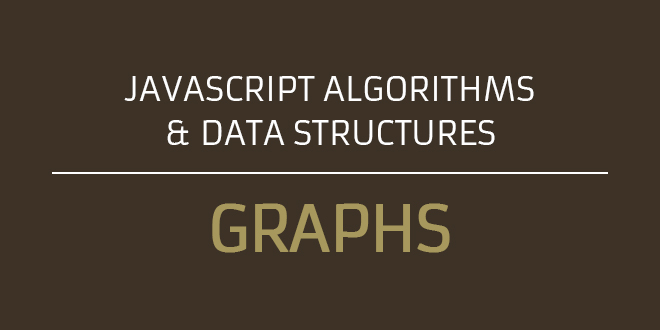
Graphs are mind blowing! The first time i studied graphs and its applications, i was simply in awe. The first thing one might think when they hear graphs is to think of some kind of chart or diagram. But that is not the case. They are actually derived from the study of networks and are an extremely hot topic these days. We have all used graph applications without even realizing it. Social media and social networks (Facebook, Twitter, Instagram, etc), the internet, etc. are applications of Graphs, and are used to model many real world systems, like airlines, road traffic, communication, etc. Graphs also fall under the non-linear data structures, but take things to a whole new level. You can even think of linked lists and the binary tree data structure as a form of graph (so we have been using graph applications without even realizing it). Linked lists have node connections from one node directly to another node, and binary trees have one node which could potentially connect to 1 or a maximum of 2 nodes. With graphs any node could potentially link to another node within the collection. So it is not limited as linked lists or Binary Trees. Lets look at our first graph.

In our collection, look at the link between the nodes. K is linked to T, M and J. Notice that M has a link to all other nodes. This is how social networks are built. Lets transform this diagram again.

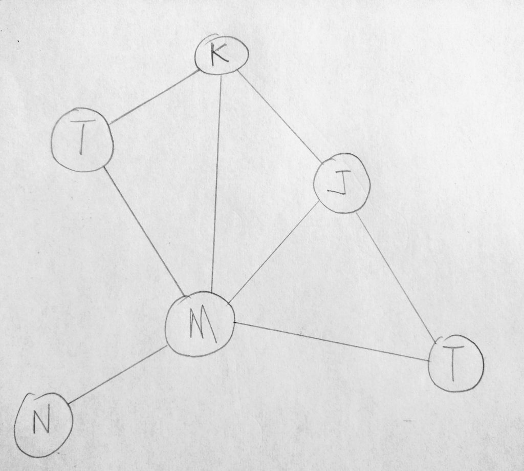
In a social network like facebook, friends have connections. Kofi is friends with Tani, Max, Julie. However he is not directly linked to Tarik (thus they are not friends). Then facebook decides to use the fact that 2 friends of Kofi (Julie and Max) are friends with Tarik, so lets us “suggest” Kofi to be friends with Tarik (chances are they know each other). See the potential power behind graphs? Behind the scenes we have enquire many things about the nature of our graph, and use that to solve other problems. We haven’t even scratched the surface of what graphs are capable of. Before we dive deeper, lets look at some graph terminology.

Terminology and Definitions

The idea of graphs are derived from theories in mathematics. So you are most definitely going to be hearing some mathematical terms. But worry not, because everything is going to be explained to you (i will do my very best). Lets look at a diagram.

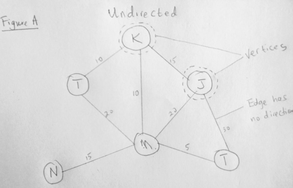
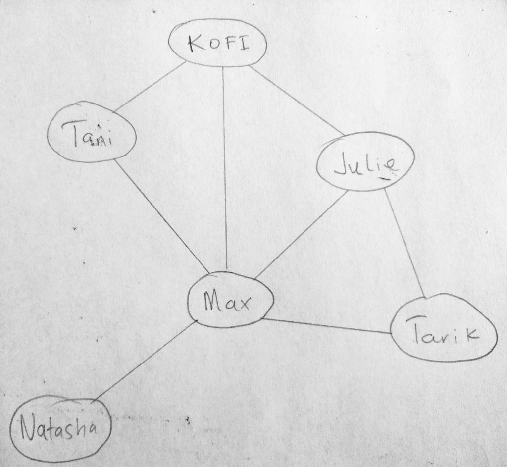
We have already looked a diagram similar to figure A. Only this time we have added some labels to it. So far in our studies in data structures, we have talked about collections of nodes. In graphs, nodes are called vertices (and a node is called a vertex). So we will not be calling them as nodes anymore. The link between two nodes is called an edge. Notice that the edges in this diagram do not have direction. Graphs like these are called undirected graphs. Let look at a diagram with edges that have direction.

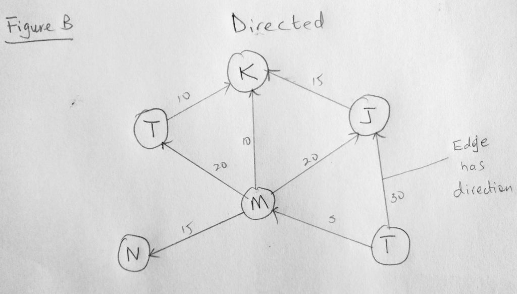
See what i mean? The connection between two vertices here has direction (things can only flow in one way). In figure A, there is no direction, so it means you can move in either direction. Notice that both figures also have numbers on the edges. This is optional. Graphs that have these numbers are called weighted graphs. These numbers are sometimes used to calculate for e.g distances between cities or even streets (it could be anything really, as long as there are edges between the vertices). The number could even represent priority, in say a navigation system, where a higher number means a more/less reliable route. Notice that not all vertices in our figure has edges. If all vertices are connected by an edge, we call that a path. Other terminology you might hear are cycle, strongly connected graph, etc. A cycle is a path that starts and ends at the same vertex. If there are no cycles its called acyclic graph(the above diagram is such). A directed graph with no cycles is called a directed acyclic graph (DAG), and many important problems can be solved if the graph is represented this way.

I mentioned that linked lists are implementations of graphs. So a singly linked list would be a directed graph, where a doubly would be an undirected graph. It is also worth mentioning that you wouldn’t find a graph class in your programming language. If you are using C, Java, C#, Ruby, Python etc there is no Graph class. However you will find implementation of it, like i mentioned with Linked Lists, binary trees etc. They are all derived from this mathematical concept!

Now that you have an idea of Graphs in mind, how would you implement your own Graph? You could look into the real world and try to model objects in terms of Graphing terminology. Think of the country you live in for example. Your city could be a vertex and the roads could be edges.. With that in mind you can visualize different roads having certain weights when you connect the vertices. If i had New York and New Jersey in mind, i could represent those as vertices and I-95 to be the edge connecting the two states(as one potential route – weighted). The weights could even be a presentation of speed limited factored into the algorithm to determine best route for journey. Airline flight systems can be modeled based on graphs, where the edge (perhaps distances between cities can be factored into how much the trip would cost, or even how long the journey is). Other great examples are local area networks (LAN) or wide area networks (WAN). Remember the internet is an application of graphs. Where routers that sit on a network can communicate and route messages to other networks. If one router were to go down, graph algorithms are used to determine closest neighbor routers that can be communicated with instead. In other words the shortest distance between vertices can be calculated and much more (we will learn about shortest path soon). Do you see more potential with this data structure? Its applications are vast and truly endless.

Graph representation

In all the data structures we have looked at in this series, we have always found a way to represent it by class. That representation was based on the way we described things for the structure. Lets find a way to describe Graphs so we can write code that describes it. It turns out that there are 3 ways: Adjacency Matrix, Adjacency List and Adjacency Set. We will not be a talking about Adjacency Set in this post (same as an adjacency list only using sets). So what do we know about a Graph? We know that within a graph, there are vertices. We also know that there are edges between these vertices (remember vertices are like nodes in a collection). Take facebook for example, a vertex could be your friend (with a name, gender and other properties). An edge however connects two vertices. It is an ordered pair represented in the form (u, v). This means that there is an edge from U to vertex V. Remember the edge in a graph system (depending on that system) could represent things like, a distance, cost, value etc. It is worth knowing that in a directed graph, (u, v) is not the same as (v, u). This is because the cost of going from A to B might be different than going the opposite way. This is not so for undirected graphs, in which case (u, v) is the same as (u, v). The direction plays a role. In undirected graphs, it works both ways, but for directed graphs it works only one way (depending is where the direction is pointed to).

An Adjacency Matrix is simply a 2 dimensional array. And as you already know a 2D array is organized as a matrix, with a number of rows and columns. In this matrix, if there is an edge from u to v, we represent it with 1, and zero if otherwise. So having adjMatrix[u, v] = 1 means that there is an edge from u to v. And adjMatrix[u, v] = 0 means there isn’t. Take a look at a diagram below.

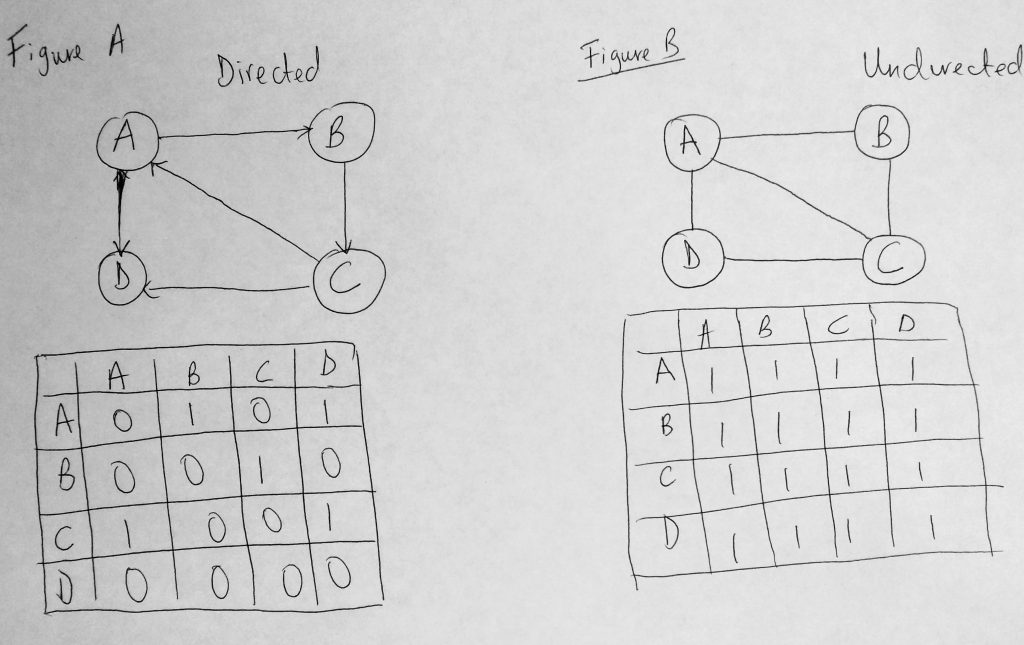
Above we have figure A and figure B which represent a Graph (directed and undirected). We have our edges represented as well (1’s and 0’s). Notice that in the directed graph (figure A) that (A, B) is 1 and (B, A) is zero if you follow the direction. But for the undirected its 1 in both cases (undirected graphs said to be always symmetric). It should be noted that working with an Adjacency Matrix, turns out to be not efficient as it consumes a lot of memory, and has a space time complexity of O(V^2). Adding a vertex to the structure is O(V^2). Removing on the other hand is O(1). You can dive more into writing this implementation if you want but we wont be doing that in this post (perhaps i might consider adding this later on in the future). We will favor the Adjacency List approach instead and write our class based on it. Please note that you might also want to consider using an adjacency set instead of a list. The set is faster than the list, but a list makes it easier to teach the concepts. They do the same thing, only one might be a bit faster.

In an Adjacency List, all vertices that are connected to another vertex are stored in a list (called adjacency list). So in an adjacency set, set use a set. For an adjacency list, we can use an Array, Linked List, Dictionary/Map, etc to store the list of adjacent vertices. Think of it this way, for each vertex we use a linked list (or array, or other data structure) to store the connected vertices. Look at the diagram below:

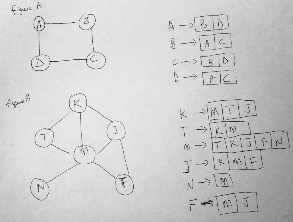
I hope you see what is going on in this diagram. The list in Adjacency list comes from the list you see connected to each vertex. In figure A for example, B & D are connected to A. So you see to the right of diagram that A -> B, D. The Adjacency list of A is B & D. Notice here that the diagram is an undirected graph. What is it was a directed graph? Let try to picture this. Suppose in figure A, the vertex A has an edge pointing to B and D, then we would have A -> B, D. Next we have a edge, from B to C. Since there is an direction from A to B, B now only points to C. So its adjacency list will be B -> C, and NOT B -> A, C like we have in the diagram above. Lets write a basic class structure.

The Graph Class

Lets write some code !

See the Pen Javascript Graph – Base by kofi (@scriptonian) on CodePen.

The class above describes what we have been talking about Graphs. Within our class we have two properties, one for vertices and the other for our adjacency list (which holds our edges or connections between vertices). Notice that we store our vertices in an array. Since each vertex has an adjacency list, we use a map to store the vertex name as the maps key, and the value will be an array (holding the list). That should be easy to understand.

addVertex & addEdge

Next lets implement methods that enable us to add vertices and edges to our Graph.

See the Pen Javascript Graph – addVertex & addEdge by kofi (@scriptonian) on CodePen.

addVertex takes a vertex that needs to be added to the graph as a parameter, and adds that to a vertices array. Anytime we call addVertex, we also want to create an adjacency list for that newly added vertex. Remember we are using Maps here as our adjacency list, so the key of the map will be the same name as the vertex passed into the function (so we can reference it by name). The value will be set to an empty array for newly added vertices. Next we have a helper method to get the adjacency list of a vertex (the one stored in the map object – Makes sense as we need to have a way to get that list for any vertex). We tell it which vertex we want by passing in the name as a key, and an array object is returned when the function is invoked. We then push onto that array (which is the adjacency list). This push is done in our addEdge method. Remember that edges connect vertices. In addEdge all we are doing is adding to the adjacency lists for any given vertex. Hope this is clear enough. Now let us test what we have built!

See the Pen OxRGmL by kofi (@scriptonian) on CodePen.

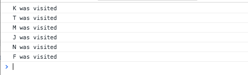
Here we put our Graph so far to the test. We instantiate a new Graph class and create an array of vertices we want to add to our Graph. We add them to the graph one by one using an array helper calling our addVertex method on each iteration. Next we setup our adjacency list by calling addEdge. Here my goal was to use the same information we used in Figure B of the last diagram, where i introduced the adjacency diagram. When we run this in the console:

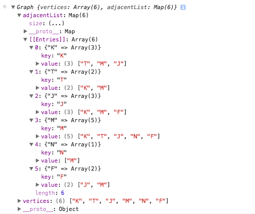
See in our Graph we have entries in our adjacency list (which is a map). You can also see that K has a list of T, M & J. This was exactly what we saw earlier. So our graph is working so far. Let us make it a bit easier to display this data. We will add a toString method to our class, which outputs all the adjacency lists within our graph.

See the Pen Javascript Graph – toString() by kofi (@scriptonian) on CodePen.

The toString method should be self explanatory even though a bit tricky. All we want to do here is go through all the vertices and output its adjacency list. But the tricky part is working with Map/Dictionaries when it comes to iteration. Look at the ES2015 and above implementation. So dead simple (3 lines of code vs 17 lines or so for the ES5 version). The ES5 version is quite complex, just to display each key with its array values. Finally here is the output of toString.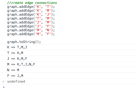

Lets move on and learn how to traverse graphs

Searching a Graph

Searching a data structure is always important, as it helps us solve problems based on the collection we have. We do this because we want to find a node(s) of concern. When designing graph applications one might want to know which routes to take to reach other vertices. For example, which roads take you to the highway (in a map application). Earlier on i talked about cycles within a graph. Our ability to traverse graphs allows us to come up with conclusions on the graph (it allows exploration). For example check to see if there are any cycles within the graph. Web crawling, friend finder, friends of friends, network broadcasting (a packet will have to explore a graph, which is the network and deliver the package to nodes on a network), garbage collection, are all graphing algorithms at play! There are two algorithms mainly used to search a graph: Breadth First Search (BFS) & Depth First Search (DFS).

Lets look at these at a high level. When searching graphs we have to have a starting vertex. From there we go through its edges and mark vertices we come across during our search. Lets dive deeper. We track each vertex that we have or have not visited. To know that a vertex is completely explored we need to look at the edges connected to the vertex. If an edge has not been visited we add that to a list of vertices to be visited later (another data structure). In a BFS we store the list of vertices to be visited in a Queue (FIFO), where for a DFS it would be a Stack (LIFO). When marking vertices, colors are used. White is for vertices that have not been visited (so all vertices are therefore initialized to white on application start). Grey for those that have been visited but not fully explored, and black for completed explored vertices. For this reason we visit a vertex at most twice to ensure its complete exploration.

Here is the difference breadth-first and depth first: In a BFS, all nodes at the same distance from the origin are visited together, whiles in DFS, all nodes in certain direction from the origin is visited together.

Breadth-First Search

Before we dive into code, i think its best to know how each algorithm works using diagrams. This is so everything is crystal clear to you before you write a single line of code. There is a lot going on here, but i think its necessary to have these here for completeness. If you want a more visual presentation check out this video, my diagrams are more geared towards examples already used in this post (but the illustrations in the video may help as well). It will be a good idea to print these diagrams, and use them as you continue reading this post.

 

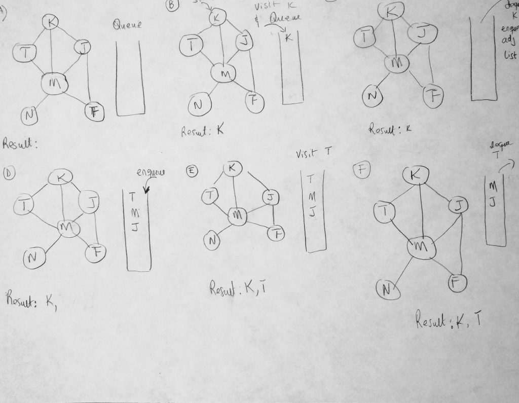
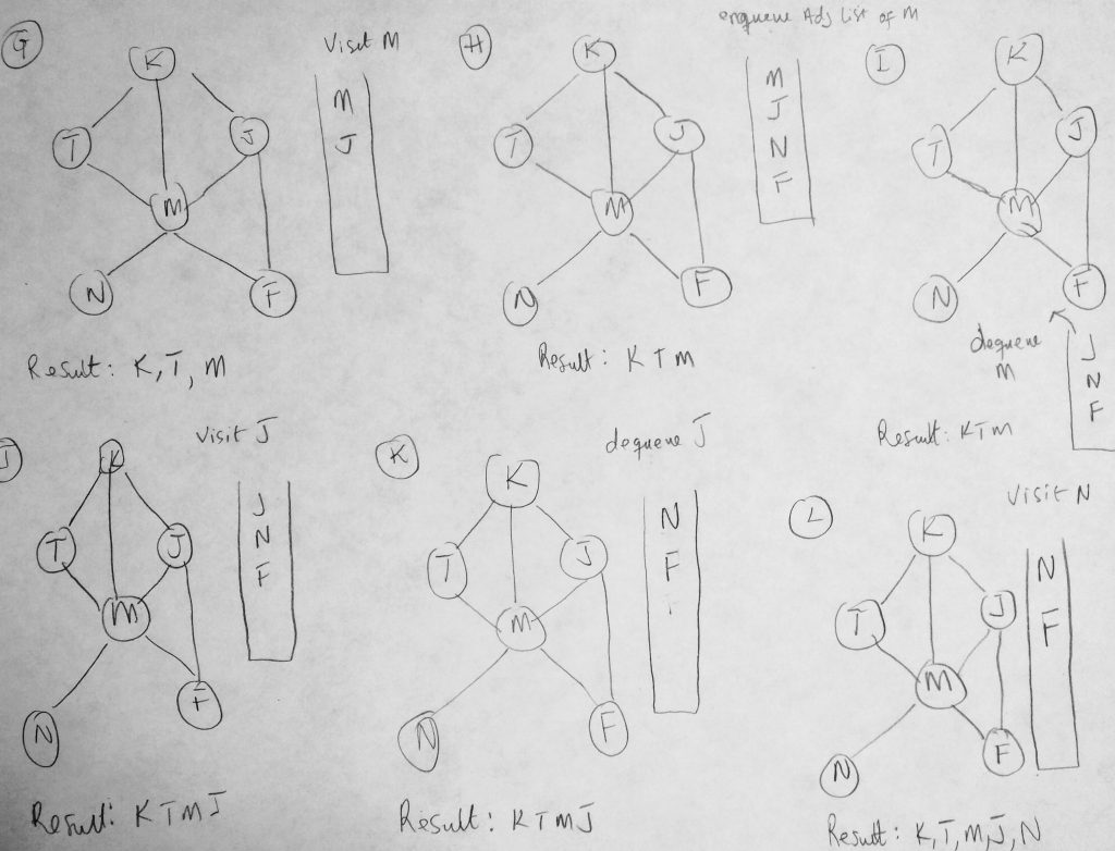
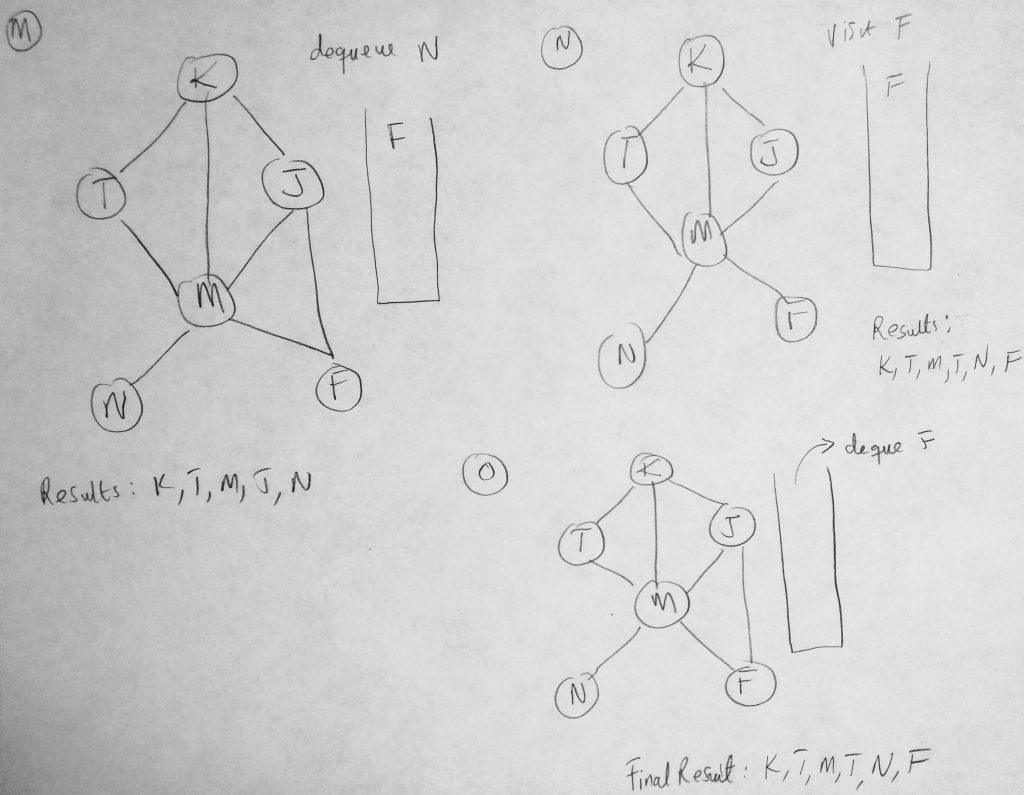
We have seen a portion of this diagram before in other examples. However this time we are using it to show you how our BFS algorithm will take place given such a graph (a step by step approach). The BFS algorithms works its way in layers (dont forget the difference between BFS and DFS). It begins by visiting a starting vertex (which gets added to a queue), and visits all its adjacency list vertices for that vertex (same level). Vertices on the adjacency list for the vertex being explored are added to the queue as they are visited and when the time is right, dequeued once the vertex is fully explored (marked completed).  In figure A we start with a clean slate. All vertices are marked as white (there are no marked colors in the diagram so bare with me here). Our search starts from K. Every time we visit a vertex we have not visited before we print the value to the console as well as mark it grey. We also push it onto our queue as well as print the name of the vertex being visited. So if its already visited we don’t push onto the queue (we will know because of color). In the figure #b, K is pushed onto the queue. From here we dequeue whatever is at the top of our queue and enqueue all of its adjacency list vertices onto our queue. We repeat this until all vertices are visited. We dequeue whatever is the at the front of the queue and perform our operations: Check to see if it has adjacency lists vertices that have not be visited and add them to the queue. When done we mark the vertex as black. Lets code BFS method.

See the Pen Javascript Graph – Breadth First Search by kofi (@scriptonian) on CodePen.

With this code implemented if we decide to traverse are Graph by calling the breathFirstSearch method, here is the output we get.

As you can see our method traverses over all vertices in our graph. Lets take a closer look at the code details. We start off by initializing some basic properties. We setup our queue and color array and we initialize all vertices in the network to have a color of white. Then we begin our enqueueing process. As long as the queue is not empty, we keep running the same logic. We dequeue what was just enqueued and get its adjacency list. We run through those vertices and enqueue only the ones that have a color of white (means its never visited). When we are done we set color of the dequeued vertex to black.

Finding the shortest path

Probably one of the most common tasks performed when working with graphs. How do we find the shortest possible path from vertex U to V? What if we wanted to find the shortest paths from vertex U to all other vertices in our graph? These help us solve problems like whats the best route to take to a destination as an example. You will find this algorithm used a lot in the transportation and scheduling industries, where it is necessary to find the most efficient route a product should take to reach a customer. Uber, Google and Amazon are big on using this algorithm (my dream companies, facebook too).

To understand the shortest path algorithm we have to understand what the distance table is. It is a data structure through which the algorithm operates through. Understanding the distance table is crucial as it is used in both unweighted and weighted graph systems for calculating the shortest path. We have not spoken much about weighted graphs, but we will be using Dijkstra’s algorithm to solve for shortest paths. This relies on the distance table. Lets take a look at what it looks like

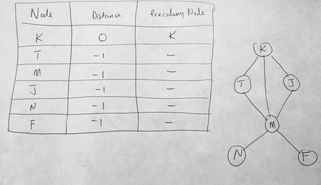
Lets talk about the distance table above. It consists of 3 columns. The first column is used to store all vertices in our graph. To the far right we see our graph system (the same one we have been using in this post). The second column hold the shortest distance from the source node to that node. In the diagram above we use ‘K’ as the source node, and since there is no distance from K to K, it is initialized with zero. The remaining distances are always initialized with infinity or -1. The third column (Preceding Node) holds the previous node we encounter before the destination node. With out table initialized let us look at our distance table populated.

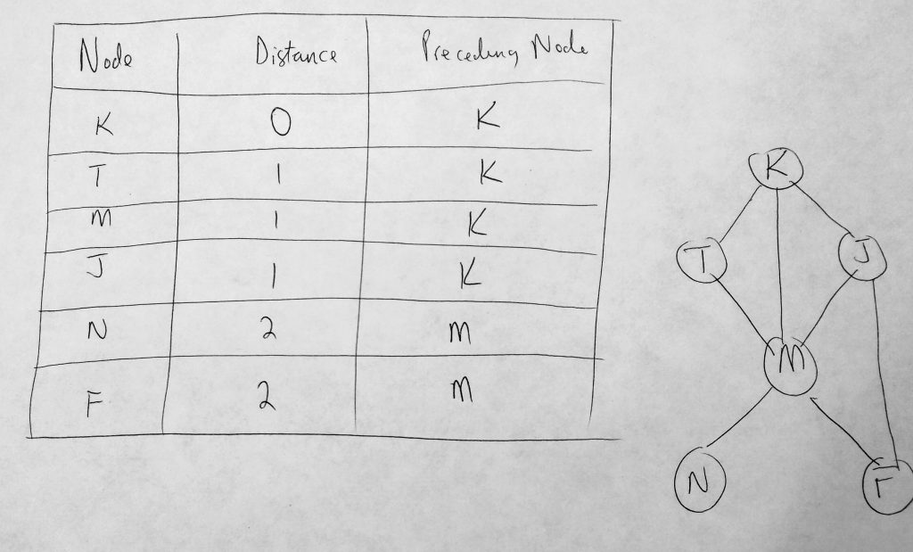
Lets take a look at a more complete distance table. In the above table, K is our source (or where we are starting from). The distance of K to K is 0, K to T is 1, K to J is 1, K to N is 2, K to F is 2, etc. In an unweighted graph we assume that the weights betweens vertices are all 1. So the distance being referred to here is the number of hops from source to destination. From K we take 2 hops to get to N, etc. Finally in our last column, where we define our preceding node, or the node that was traversed last before the destination node. Starting from K as a source, the preceding node to T, M, J are all K. To get to N or F from the source (K), we have to go through M. This is why you have the following vertices in the preceding node column. It is important to note that the distance table always have a source. So anytime your source changes, your distance table will be different.

In order to find the shortest path a method known as backtracking is employed. In order to backtrack, you are most certainly going to need a distance table for that. So how do we get this distance table from what we have done so far? It turns out that all we have to do is modify our BFS method to return the distance table data. We can use this data to help us find the shortest path. Lets look at another diagram where we want to find the shortest path from K to N to illustrate how the distance table is going to help us.

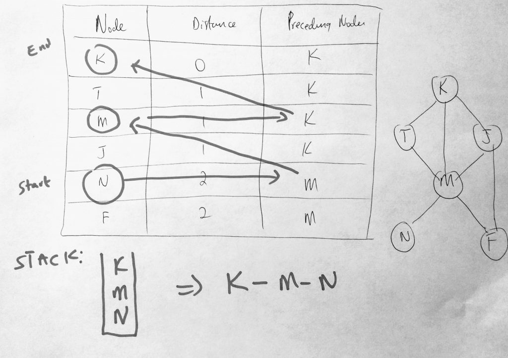
Backtracking is normally done using a stack. We start from our destination node N (which we place in the stack – remember we are working backwards, hence backtracking). As long as the source and destination are not the same, we find the preceding node N which is M. We place that into the stack as well. Then we find the preceding node to M, which is K. We place K on our stack. Then we find K and notice that its distance is zero (meaning its the source). At the point we have some items in our stack. We pop the items off and get a result of K-M-N as the shortest path from K to N. Simple right? You can choose to use an array if you like. You can push to the front of the array as you move through the distance table, or push to the back and use a method like reverse to get the final path.

I will implement 2 shortestPath methods ( how to find the shortest path from one vector to all vectors and the path from vector U to V for example (specific paths) ). Also it is worth noting that the shortest path algorithms have a few variations. There are shortest path algorithms that use weighted or unweighted graphs ( we will be looking at the unweighted algorithm — where all path weights equal 1). Lets just straight in ( here are both ES5 & 2015 versions )

See the Pen Javascript Graph – Shortest Path by kofi (@scriptonian) on CodePen.

There is a lot of code there! But we have talked about everything already. The first thing to note is how we are creating our distance table. Previously we initialize all our color to white before we did our BFS. Now we are adding to that color function and initializing the distance and preceding node tables. We set all distances to -1 expect whatever our source or starting vertex. We also set our preceding nodes by creating an array of objects with key as the vertex and its value as the preceding node. All the nodes are set to null except whatever the starting vertex is, which will be itself.  Then within our forEach method where we set the color to grey, we increase the edge distance starting from 1 if its -1 (what it was initialized to). Then we return an object at the end of our BFS which contains all the distances and preceding nodes.

We start off with the shortest_path method. This method takes a BFS because we need to use our distance table in our to find the shortest path. The method also takes the source and destination vertices. We create a stack to store our paths and begin pushing to it (see github code comments). Earlier on i said we start with the destination (diagram above), for eg if we want to find the shortest path from K to N, we start from N (adding it to the stack). Then we get its preceding node and begin backtracking. As long as the preceding node is not null or not the source, we add it to our stack. If that is not the case then chances are the preceding node is null or its equal to the source. At this point we add that to the path.  When done we pop items from the stop of the stack to get our final string. Printing the shortest path from source to all other nodes is done using the already exist shortest_path method. That method should be self explanatory (only a few lines of code). Whew, lets me on.

Depth-First Search (DFS)

DFS starts its search from an initial vertex and follows that path until it reaches the last vertex. After which it backtracks and follows the next path. It does this until all vertices are visited and there is no path left. Whiles the BFS uses a queue to store visited vertices, a DFS uses a stack for this storage. The implementation for DFS are quite similar to BFS even though the underlying data structure is different ( queue vs stack ). We can also use recursion as a way to do depth first search. I will show you both ways (and you can choose which way you like best). Lets take a look at them (in ES5 and ES2015 and above).

See the Pen Javascript – Depth First Search by kofi (@scriptonian) on CodePen.

The first thing we will talk about is the depthFirstWithStack method (since it is very similar to the breath-first methods we have seen early). It should look very familiar to you. We create an array to hold our colors and initialize all vertices to white. We also create our Stack, which is the underlying data structure we store our adjacency lists in. First we get the starting vertex and we push that onto the stack. As long as its color is not black, it means it has not yet been fully traversed / visited, we change its color to grey, get its adjacency list and put that onto the stack. We keep exploring by popping off the stack (the vertices already added) until there are no more to be explored. Every time we pop an item off the stack we add its adjacency vertices to the stack(if they haven’t already be explored).

Next, we have a recursive way of doing depth first search. The approach is split over two methods DFS and DFSTraversal. We first call DFSTraversal which does some initial setup (like we have being always doing), colors initialization etc, and then runs through all the vertices calling the DFS method. Each call to the DFS changes the state of the vertex (from se, not visited to visited), gets the adjacency list of that vertex and recursively calls the DFS method to traverse the remaining vertices.

Graphs are extremely powerful as you can see. This has probably been the hardest post for me to write (because there were so many new things to learn – the hardest part was to teach it) and we most definitely didn’t cover everything (there are entire books written on the graphs, so we cant possible cover it all in a post. I have put enough here for you to be able to answer just about any question in say an interview question, for example). I learned a lot and i hope you have too. Play around with some of the ideas we have discussed here. Try building your own graph class and maybe even extend it. Add an option to make the graph directed or even be able to specify weights when you add edges (instead of the default of 1, for unweighted graphs). With the realization of what graphs can do i am sure i will be back to write more about other applications using this amazing data struction. I think we may be able to solve many problems using graphs and they have most definitely peaked my interest (more than any data structure thus far). If you read this post, let me know your thoughts. Or if you decide to build something with it, i would love to hear! Feel free to reach out on twitter as well ( @scriptonian ) if you have any questions.

This is the last data structure in our series. We have covered it all! Lets move to the topic of algorithms!