Now that we understand dynamic programming, let’s dive into greedy algorithms. A greedy algorithm (also used in solving optimization problems) is one that builds a solution in small steps, making a locally optimal choice at each step in hopes that eventually it will find a solution that can be applied globally. So what does all this mean? We call it greedy because, at each step, it makes the most optimal choice (this is what we mean by locally optimal – meaning whatever value I have at this step, is the most optimal). It continually runs (step by step) until the best optimal solution is found overall. Greedy algorithms do not always give the most optimal solutions (they don’t always work). However for many problems they actually do (even nontrivial ones!). Sometimes, this is all you want for a given problem ( an optimal or even suboptimal solution – something that works decently). Sometimes making a decision that looks right at the moment will give you the best solution. But we know this does not always work in the real world. This is what greedy algorithms are all about.

Greedy algorithms are easier to implement than using dynamic programming when solving optimizations problems. Dynamic programming can sometimes be overkill, not forgetting its complexity (IMHO). We can use greedy algorithms to solve Dijkstra’s algorithm for shortest path (we saw this in a previous post). We can use greedy algorithms to solve minimum spanning tree, and many other problems. Remember they do not always yield great results, but for many problems they do. Take the 0 – 1 Knapsack Problem we looked at in the previous post. If you were to use the greedy approach then you would take the most expensive item first (as long as it fits), and the next most expensive item until the knapsack was full. But as you already know that won’t work here, or that won’t give us the maximum profit. However, the solution is close to the more optimal approach. Greedy algorithms may speed up the search for a solution, but the caveat is that they might resolve to a locally optimal solution that does not yield the highest maximum result. So a greedy algorithm is definitely not the “God” of algorithms. Sometimes using dynamic programming is what will yield the results you are looking for. Here is a definition for you: “Greedy is an algorithmic paradigm that builds up a solution piece by piece, always choosing the next piece that offers the most obvious and immediate benefit. Greedy algorithms are used for optimization problems. An optimization problem can be solved using Greedy if the problem has the following property: At every step, we can make a choice that looks best at the moment, and we get the optimal solution of the complete problem”.

Let’s take a look at some diagrams that will help us understand what is going on when you choose the greedy approach.

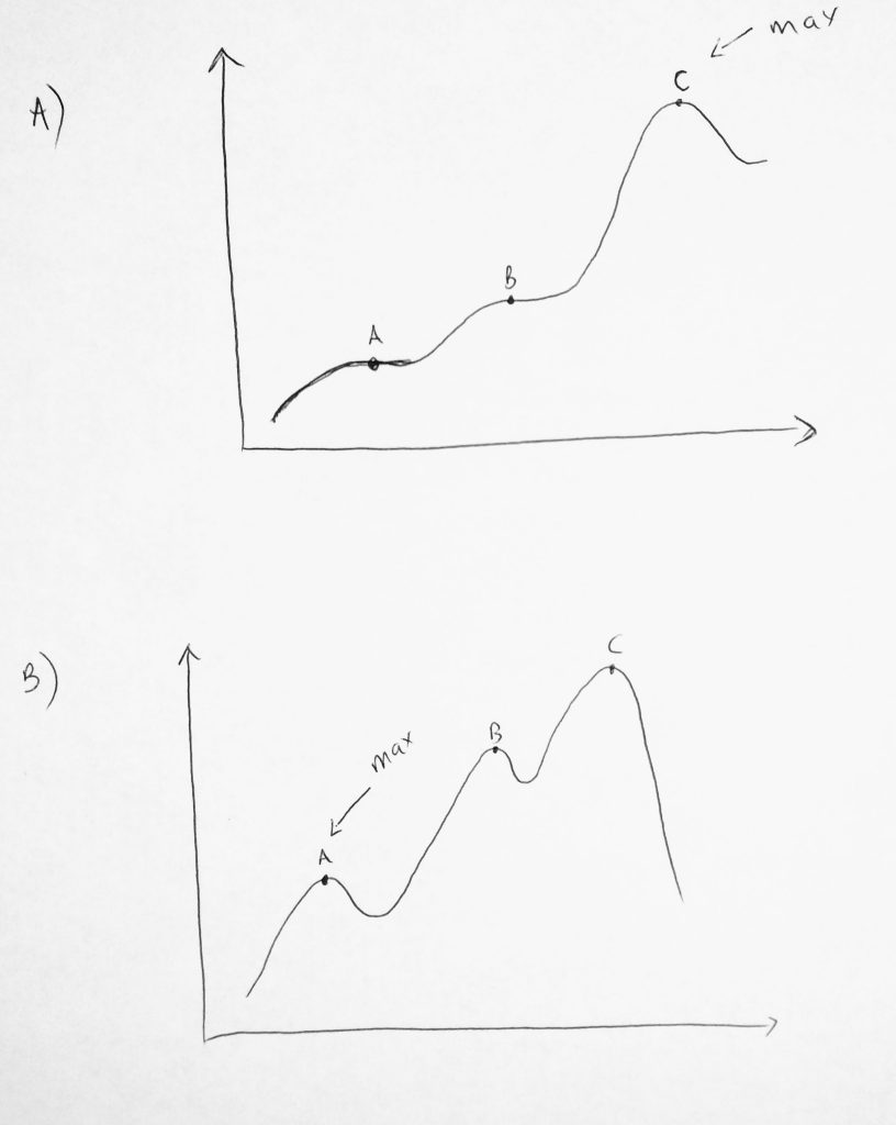
Let’s just say that the above diagram represents data points within a given problem. As the greedy algorithm runs, at each point it makes a decision as to whether that value is the most optimal (max value within the given problem). In the diagram, when the algorithm reaches a new max value on the curve at “A”, it then decides if the values after “A” are greater or smaller? Because the curve flatlines, the algorithm keeps moving forward as the curve keeps growing to a new max of “B”, then it keeps going on till “C”. When it gets to C the algorithm will stop. Why? Because if it keeps moving on, the next optimal value will tend to decrease. So it stops right there and says C is the most optimal solution.

In the diagram below A, we have another curve. However, noticed that optimal solution is at point “A”. When the algorithm gets to this point it stops! Why? Because moving forward the data values on the curve decreases. Because of this, it returns “A” as the max value. Now is this optimal? No, it’s not. “C” is the highest point in that second curve. This is why greedy algorithms do not always give us the most optimal solution. At each point during execution that locally optimal solution is picked. It is a local maximum and not a global one. Let’s look at the next diagram

Let’s take a look at this graph and how a greedy algorithm would approach it. Imagine that this is a graph that represents roads or cities. If you want to learn more about graph algorithms, please check out this post. In this graph, we are trying to use the greedy approach to find the shortest distance from starting point to the endpoint (shown on graph). Notice that when we start the greedy approach would try to take the shortest path. Moving in the “right” direction, which is 2 instead of left which is 7. The path it takes to get to the endpoint is

2 -> 4 -> 3 -> 4 -> 4 -> 6 ->

This is because everytime it reaches a node, it makes a decision on which path is the shortest. As you can see this will not be the most efficient route which totals 23 (adding the path values). However, the shortest path is through 7 -> 9 to get to the endpoint. A total of 16. The greedy algorithm yet again reached a local max and not a global one. We always need to make sure each step is an improvement towards the final step. If this is not done, a globally optimal solution will not be reached.

Let’s take a look at one last example

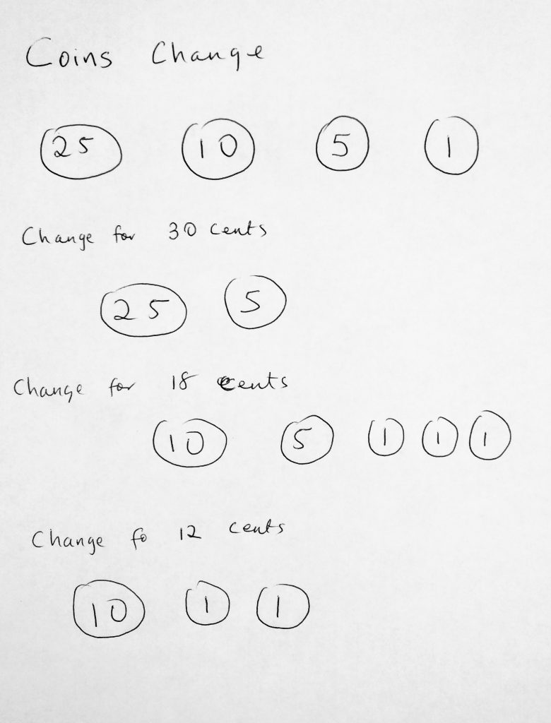
This example is a very classic one of using greedy algorithms. It’s the example of a coin changer problem. Imagine you have to give change to a customer at the register. If the change was 18 cents, then the greedy algorithm, in order to give the least amount of coins would first start with the highest possible amount. In this case for 30 cents, it gives out 2 coins. For 18 and 12 cents, it gives out 5 and 3 coins respectively. However, those apply to the united states. What if we had a coin system with the following values – 10, 5, 4, 1; and we are asked to return 18 cents, what would the greedy algorithm do? It would give you, 10 -> 5 -> 1 -> 1 -> 1, which is a total of 5 coins. However, the most optimal solution would be 3 coins ( 10 -> 4 -> 4).

Greedy algorithms may give us faster results, but you should be aware of their caveats: they might stop at a local maximum in some cases. It is important to be mindful of this.

Lets starting looking at some code example.

The coin changing problem

In the last diagram, we see how we can use greedy algorithms to solve the coin change problem. Let’s take a look at how we would implement this in code. It is much easier to do than dynamic programming. It’s pretty straightforward and intuitive.

See the Pen Greedy Algorithms – Minimum Coin Change Problem by kofi (@scriptonian) on CodePen.

Let’s go over this code. We have a class called Minimum Coin Change that we pass into the coin system we want to use. In this case, we are basing it on the US coin system (quarters, dimes, nickels and pennies). In the code, we have two functions: one to generate the number of coins given the cent value, and the other to only display the results. Note that there isn’t anything special going on here. We don’t have any recursions or storing initial values in array tables etc. It’s straightforward code. The generate coin function takes the amount you want to convert. Runs a loop based on the coin system and does basic math operations to return how many of each type we have. The display results function only outputs the results. You can feel free to modify this example to suit your needs. Let’s move on.

Fractional Knapsack Problem

In the previous post, we talked about the 0 – 1 knapsack problem. In there I explained what 0 – 1 in knapsack meant. Let’s look at a non-discrete knapsack problem. And what does that mean? We will see how to solve the knapsack problem with items that are continuous in nature. I am not going to define the knapsack problem again here. You can find out what it is in that post and then come back to find the greedy approach to solving it. Let’s reconsider a diagram from that post

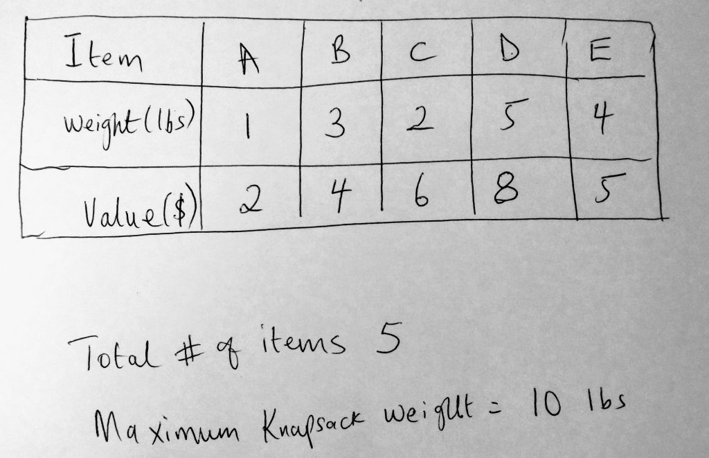
Here we have items A through E. Note that the total items we can put in our knapsack are 10 lbs total. If we were using the greedy approach (recall the diagram we spoke about), we take what we have in the given situation (local maximum). Say we can get another max moving forward then we keep doing that. If moving forward means we get a smaller value, then we stop right there. In the diagram above, the greedy approach would start by stealing all of item A, B, C. At that point the knapsack is 6 pounds with a value of $12. Notice that it cant steal all of item D, that would exceed the 10 lb capacity. However, imagine that we change what our knapsack capacity is to 12 lbs. We would now be able to steal item D, but not item E which weights 4lbs. The sack can only take 12 lbs now, taking the item E means we need a capacity of 14 lbs. However what we can now do in this fractional approach to the knapsack, is to steal a portion of E! A fraction is a portion after all. Our knapsack is now 11 lbs and we need 1 pound more. So how about we steal 25% of item E? 25% of 4 pounds is 1 pound, which gives us a value of $1.25 to make a total of $21.25. Voila! we have a full knapsack and we can run away happy. Let’s take a look at the code

See the Pen Greedy Algorithms – Fractional Knapsack by kofi (@scriptonian) on CodePen.

This structure of code should look pretty familiar if you have looked at the dynamic programming code we wrote in the previous post. However, you notice that the greedy approach much simpler. We have a function that takes 4 parameters. You may want to refactor this after 4 is a bit much. You can condense it into one object with properties instead. For simplicity sake, I have 4 parameters. The function declares two inner variables. One to keep track of how much value we have in the knapsack as we keep adding, and the other, to keep track of the weight. Then we beginning our iteration. Notice that our for loop keeps running with a special condition of whether the current knapsack weight is less than the total capacity. This is simply before if we can add more to the knapsack then why not? Within the for loop, we check if the current weight being added is less than or equal to the total capacity minus the current knapsack weight. The reason, here again, to make sure we do not exceed the capacity of what can be added to the knapsack. If we do exceed it then we hit the else clause and perform a final check. Notice that we return the value of the knapsack the moment the else clause hits. This is because at this point we have just one item to evaluate. We perform some simple math to get the remainder and percentage values of how much weight and its value to fill the knapsack up. I have a lot of comments in the code so you should be able to understand fully what is going on.

Spanning Tree algorithms

You might be wondering where else we can use greedy algorithms. Spanning tree algorithms ensure that all nodes in a graph are connected by one edge. I mentioned in the beginning that we can use greedy algorithms to solves minimum spanning tree problems. In the study of graphs, minimum spanning tree algorithms involve finding the shortest paths that connect all nodes in a graph. If anything in this section sounds foreign then I suggest you read my graph post before continuing. There can be many paths within a graph that connect nodes, but the path with the shortest weight is the minimum spanning tree. One thing to note about spanning trees is that they do not have any cycles, and one can reach all nodes from any given node.

Let’s say you want to find the cheapest way to interconnect cities with transportation links, then the minimum spanning tree algorithms are what you will use. Two of these algorithms are Prim’s and Kruskal’s. Now, where do greedy algorithms come into play? Both Prim and Kruskal are greedy algorithms used to find the minimum spanning tree for a weighted undirected graph. The only difference here is that Kruskal’s can also be used for disconnected graphs where Prims cannot. Let’s take a look at the two.

Prim’s Algorithm

Prim’s algorithm works only with weighted connected graphs. It is a greedy algorithm that is used to find the minimum spanning tree for a weighted undirected graph. Recall that all greedy algorithms could potentially result in a local instead of a global optimum value. This is true for Prim’s algorithm as well. Let’s take a look at a diagram.

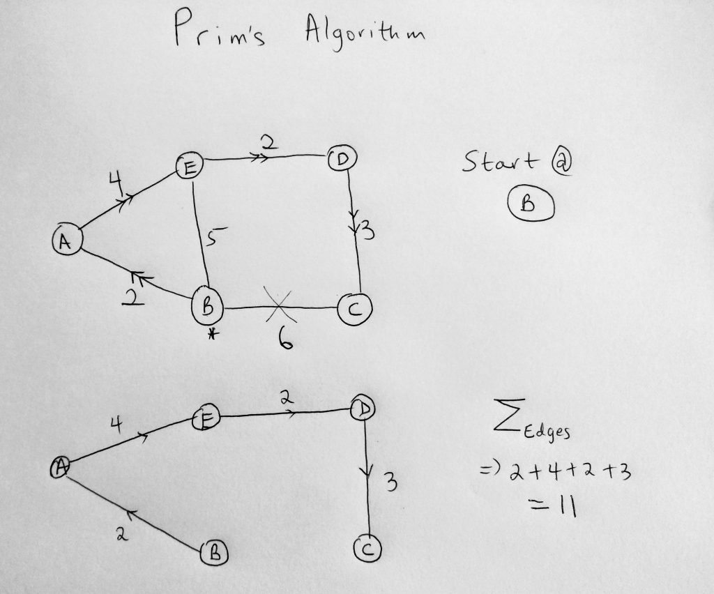
Let’s use the graph diagram above to understand prim’s algorithms. We start off by choosing any node we want to start from. In this case, we start on B (notice the asterisks). What we are trying to do is find the shortest path that will link us to all nodes within the graph (as long as they have not been already visited). Started at B, we have two paths to take. Go to A or C. But using the greedy approach, we will take whatever is the local optimum. Since that is 2, we take the path to A. At A, the most logical next step is to move to E since we cannot go back to a node that is already visited (B). The same is true when we get to E, we move to D because B is already visited. We keep doing this till we get to C (algorithm choosing the shortest path). When we get to C, the algorithm ends. Remember the number of edges within a spanning tree will be the number of nodes minus 1 (N – 1). If there are 10 nodes within a graph, then the spanning tree will have 9 edges. Summing up the edges we get 11, which actually turns out to be the true glocal optimum for this graph. Again remember this is not always true using the greedy approach. In this case, we are lucky to get a truly global minimum (which doesn’t always happen with greedy algorithms as we have seen)

Kruskal’s algorithm

Kruskal’s algorithm, just like prim’s, works with weighted connected graphs. However, it kicks things up a notch by working with disconnected graphs as well. Let us consider the same graph from before and see how Kruskal’s algorithm would approach finding the minimum spanning tree.

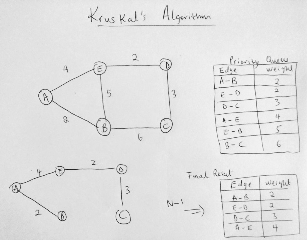
The first thing the algorithm does is access each edge in the graph and adds it to a priority queue (in increasing order of weights). Locate the queue on the right side of the diagram. Note that because this is a priority queue when edges are getting added, they are done in an order. From highest to lowest. In this case, the lower the weight, the higher the priority. The next thing the algorithm does is push a set of edges into a result, by iterating through the priority queue (results are below the priority queue in the diagram). As long as that edge does not form a cycle then it can be added. This process keeps going until we have N – 1 edges. At the point, the algorithm is done. Notice that if we add E – B or B – C, which you see in the priority queue, it will form a cycle. So it only makes sense that the algorithm is smart enough to do this. This is how Kruskal’s algorithm works.

I have not added the implementation of Prims and Kruskal’s algorithm here, however, you might find it in my Github repo in the future. If you don’t, kindly reach out to me.

I believe this is the last post in the javascript data structures and algorithms series. I have learned so much in the past year. It has been overwhelming, yet enlightening and I look forward to applying all this new found knowledge. If you have been following me all along, I would love to know how you have used this too. If you feel there is a topic left out, or that I should have covered, please comment and I will do my best to reply as soon as I can. Thank you and happy coding!

I-am Konstantin