
In a previous post we learned about searching algorithms. We also learned that sorting is equally important; that sorting and searching go hand in hand. Sorting is deeply embedded in everything we do. Lets define sorting even though we all know what it is. Sorting is simply rearranging elements in a collection in increasing or decreasing order based on a property. That property could be a datatype like string or number. We could even sort based on some complex datatype. So if you have a class with many different properties, we could sort based on those properties. In the real word, we sort cards when we play poker, when buying online we like to search in order of price (sorted from lowest to highest or vice versa), or perhaps even sorting by product number reviews (my favorite type of sort when shopping on amazon). We sort emails, phone contacts, travel dates (you get the picture).
Please find github repo here:
Normally you learn about sorting algorithms before searching, but i took a little backward approach to this. Remember i mentioned that if we can sort our data first, then searching could become easier (like we can search faster using binary search – which only accepts sorted data). I also did mentioned that sorting could be an expensive task (so you need to understand when to sort before searching). It also depends on the sorting algorithm being used as well (as there are many different sorting algorithms). We will be looking at some of them (in increasing order of difficulty). We start from the slowest, to the relatively fast and faster algorithms. So why would we ever want to implement the slower algorithms? Well when you start learning algorithms in general, its a great idea to see how they evolved over time (as humans we are always on a search for better ways of doing tasks). You get to see patterns which later help you in your software engineering career. This greatly increases your chance of writing better algorithms in the real world. It’s a good learning tool. These days there really aren’t a lot of use cases where you would use a bubble sort for example (which is the slowest sorting algorithm of them all) – perhaps when the dataset is extremely small you “could” use bubble sort. But for even such small datasets, there are other algorithms one could use that are better than bubble sort (we will learn what bubble sort is soon). In any case, lets learn them anyway – BECAUSE WE CAN, and because we are thirsty for knowledge! In this post we will learn to implement the following sorting algorithms: bubble, selection, insertion, shell, merge, quick and heap. Other sorting algorithms are counting and radix sort (we will not be covering those – as they don’t offer us any advantage over the ones we will implement in this post).
For every sorting algorithm we look at, we will discuss certain parameters, such as time complexity (Big O notation), space complexity (how the algorithm uses memory). We may also talk about how stable the algorithm is, and also whether its recursive or non-recursive. Lets jump into sorting algorithms and how to implement them in javascript.
Basic Sorting Algorithms
The first three sorting algorithms we will be looking at, in terms of in order of complexity and performance are: bubble, selection and insertion sort. These are considered basic sorting algorithms. Lets get right into it.
Bubble Sort
The simplest sorting algorithm you could ever implement is a bubble sort. Given a collection of data, we iterate through the entire set multiple times. On each pass through, we perform certain actions. First we check to see if the current item we are on (during the iteration) is greater than the next item in the list. If it is, we swap the current item with the item in the next slot, if not we don’t perform a swap. We keep performing this action until there are no swaps for a given iteration. This swapping action causes a ‘bubble’ effect, shifting or moving the highest values towards the end of the collection. In the first pass, the highest value is pushed all the way to the end. In the second pass, the second highest is moved, etc etc until the collection is fully sorted. Lets take a look at a diagram
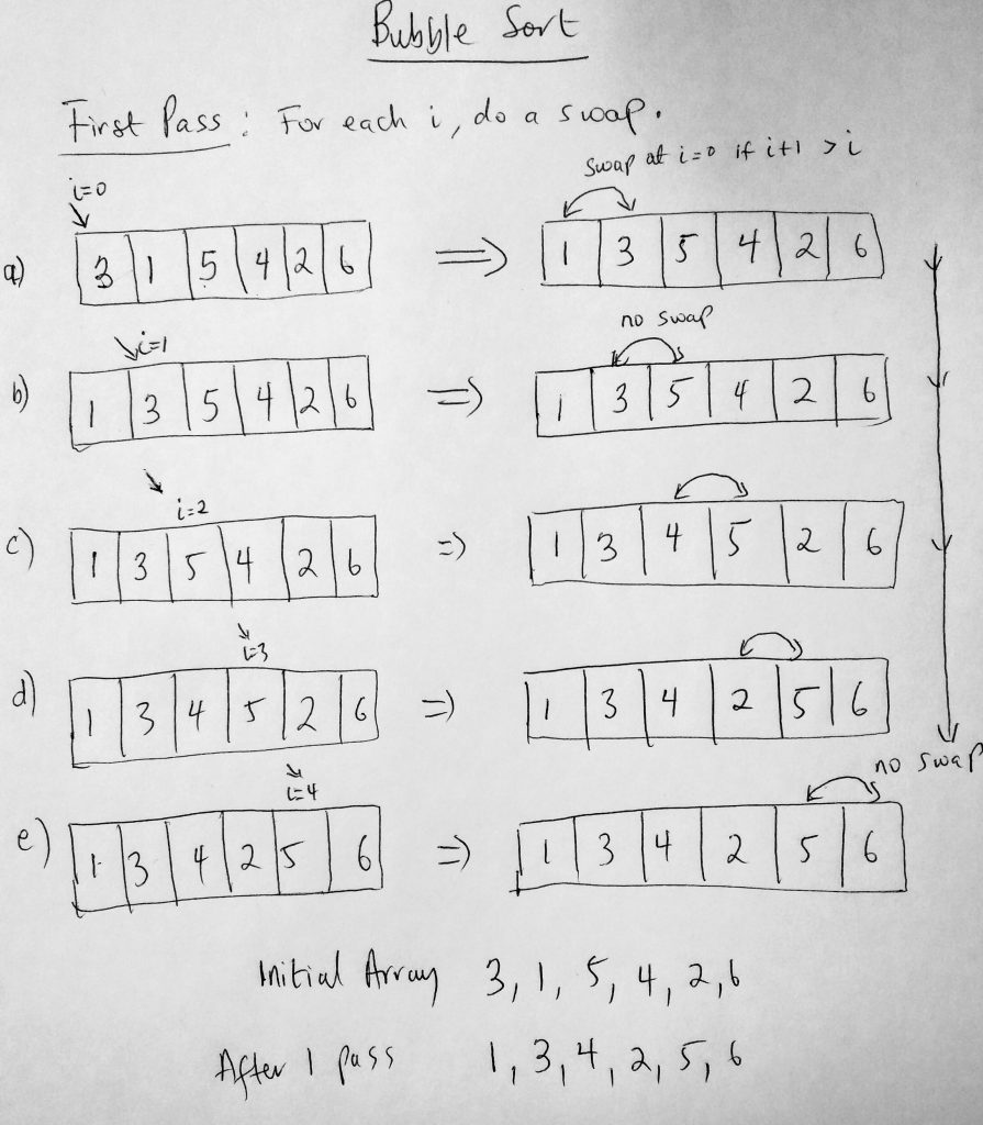
In the example above we look at what the first pass looks like; we are given a dataset to sort (from lowest to highest). The initial state is [3, 1, 5, 4, 2, 6]. At the end of the first pass, we notice that we get [1, 3, 4, 2, 5, 6]. Normally in the first pass, we get the highest number in the collection pushed to the end. We already had 6 at the end in the initial array so that didn’t change, however the next highest (5), bubbled up next to the 6. Think of it this way, given an array [3, 1, 5, 4, 2, 6], we start from the index 0 (3). There are 6 items in the array so we make 6-1 = 5 passes (since by the last one the data is already sorted). We compare all values in a slot with the next value and swap. We keep doing this till we reach the index – 1 value. Now here is a tip i don’t see many do when coding bubble sort: The moment there isn’t a swap in any iteration, it means the collection is sorted, and you can stop execution right away. This will actually make your sorting algorithm faster IF you check for this condition. Lets start writing some code.
See the Pen Bubble Sort by kofi (@scriptonian) on CodePen.
Lets go through this code. I have created Scriptonite Sort, which is a javascript sorting library. Its a simple library for testing different sorting algorithms – a work in progress and will be the theme for this post :-). In this library we will be able to call all sorts of sorting algorithms. We will start off with bubble sort. I have created two bubble sort functions (a basic and enhanced version). Lets dive into the code. The function takes two parameters, the first is the data list that needs to be sorted. The second parameter is optional (a boolean value of whether or not to show logging to the console). We assign the passed in data list to our parent class’s array variable. This ensures that anytime we call a new sorting algorithm (for eg insertion sort) with a new data list, that list will be used instead. Other variables declared in this function are the number of passes and the length of the passed in array. Since bubble sort works by processing the data list in multiple pass, number of passes keeps tracks of how many times it takes before the collection gets sorted. So, what happens on each pass? Here is how the algorithm works. We iterate through each index in the collection, from 0 to n-1. And for each index we perform our pass through algorithm. When we are on index 0, we just to see if index 0 + 1 is less than index 0. If it is so, then we call a swap function to swap those two index value. For e.g. if we had [2, 4] then after we swap, it becomes [4, 2]. We keep doing this till we get to the end of the array, then move to the next iteration in the outer array. Finally when all passes are done we output the number of passes and the result of the sort to the console.
The second function (bubbleSortEnhanced) tries to improve on the algorithm. It is very similar to the first but it adds a few more functionality. The first thing is does well is try to avoid unnecessary comparisons. Lets talk about this in detail. Lets just say that after a few passes, you have a collection that looks like this [1, 5, 3, 7, 8]. We bubbled 8 and 7 to the end of the array. On the 3rd pass, after we swap 5 and 3, is there really a need to compare 5 & 7? Or 7 & 8? No we don’t need to compare them again. So this second method takes that into account (because its not needed – its already sorted). Another very special thing this next function does is to take into account that if an array that is already sorted is passed into the function, that it will make only one pass and not multiple. The trick here is to understand that during your iteration, if a swap never ever occurs it only means that the list is sort. So i set some boolean values to handle whether a swap has occurred or not.
Bubble sort is not a great performing algorithm, so i would recommend using it in the real world (there are better algorithms). The worst case performance for this algorithm is O(N^2). Its not good if you use this algorithm for large data sets. Since we have already learned that the N in the Big O notation is number of operations. For a data set with 10 items, bubble sort would perform 100 operations to get it sorted. As the data set grows, the number of operations grows exponentially. If you sort a thousand items it could take 1 million operations in the worse case scenario. So as you can tell, its really not great for large data sets. Now this does not just apply to worse case scenarios, even average case scenarios would still perform at O(N^2). However thing start getting better if you smaller data sets. We can actually get a runtime of O(n) with such small collections. If the collection is sorted or nearly sorted, we can actually get good performance out of this algorithm. And yes even if the data set is large and data almost sorted or already sorted, bubble sort works at O(n). In terms of space complexity, the operations performed did not require any extra memory allocation (this is what we call “in place”). Big O for space complexity for bubble sort is O(n) because of this. The number of operations here only depend on how large the data set is. In terms of stability, it is considered a stable sort. If you have two elements in a certain order in your collection, that ordering will be maintained in the sort (the the nature of the swaps). This is what we will refer to as stable when it comes to other sorting algorithms.
Thats about it for bubble sort. Lets move to the next sort algorithm – Selection Sort.
Selection Sort
Selection sort is very similar to bubble sort. Whereas bubble sort pushes the highest items in the collection to the end of the array (via swaps and comparisons), selection sort does the opposite of pushing the smallest items to the beginning of the array. Think of it this way, find the smallest item, put it in the first index (0). Find the second smallest and put it in index 1. You keep doing this till the collection is sorted. Selection and Bubble sort have pretty similar performance. Both worst and average case performance are O(n^2), however selection sort performs better that bubble sort in the average case scenario due to fewer swaps used in the algorithm. Matter of fact we don’t do more swaps that the total number of items in the collection (which is not the case for bubble sort). Finally the best case scenario is O(n^2). This is due to the many comparisons done in the algorithm. One needs to consider the system they are operating on. How cheap or expensive is it to do comparisons or swaps. If its cheap to do comparisons, then perhaps this algorithm is for you. The space complexity for selection sort is O(n) (that is, in-place). Lets take a look at a diagram.
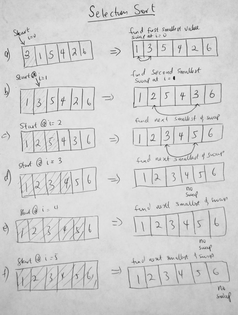
Here we can see what is going on in the algorithm. In figure a, we start with an array with 6 items. We start at i = 0, we take that number and compare it to all the numbers in the collection in hopes to find the smallest number. When we find it, we place that number in index 0 and place what was originally at 0 into where we found the number (see diagram). We keep doing this until collection is sorted. Notice that in step d, e and f, we don’t do any swaps at all, however we still do comparisons. Lets take a look at the code in action.
See the Pen Selection Sort by kofi (@scriptonian) on CodePen.
Lets see what is going on in our code. This method is very similar to bubble sort. So i will skip explaining everything. Like the bubble sort, we will also have a nestor loop. The outer loop keeps track of the index that needs swapping. For example, if index 0 has the value of 9 (outer loop), the inner loop goes through all values in our collection and keeps track of what the smallest number will be. That smallest number is compared to the 9 value. If its smaller they are swapped, if not then its not. Thats pretty much what this function is doing. At the end we return or console log the array from smallest to highest. As you can tell, there are lots of comparisons done here and fewer swaps. I have also provided the ES2015 & beyond version in my github repo. So check that out if you are more interested in that version. Finally i should mention that selection sort is not a stable algorithm. And if you read the chapter on bubble sort you should understand what this means. So item of the same values might be rearranged when sorting happens.
Insertion Sort
The final basic sorting algorithm we will talk about is the insertion sort. This algorithm is a little more performant that bubble and selection sort. That said it is still a very slow algorithm (all basic sorting algorithms are slow – this one though is the better of the three). Insertion sort is one of those algorithm that feels very intuitive. One can say it is analogous to the way humans sort data. Imagine having a deck of cards in one hand, say the right hand. You decide to sort the cards in increasing order so you start putting those cards in the left hand one by one (in increasing order). That means that you sort the collection as items are encountered. If you have 3 in the left hand, and you pick a 7, you automatically know that its bigger than 3 so you insert it to the right of 3. I guess we now see where the insert in insertion sort comes from. On one side we have the unsorted part, and on the other side we have the sorted part. We remove an item from unsorted over the the sorted part and insert it in the right location. Lets take a look at a diagram.
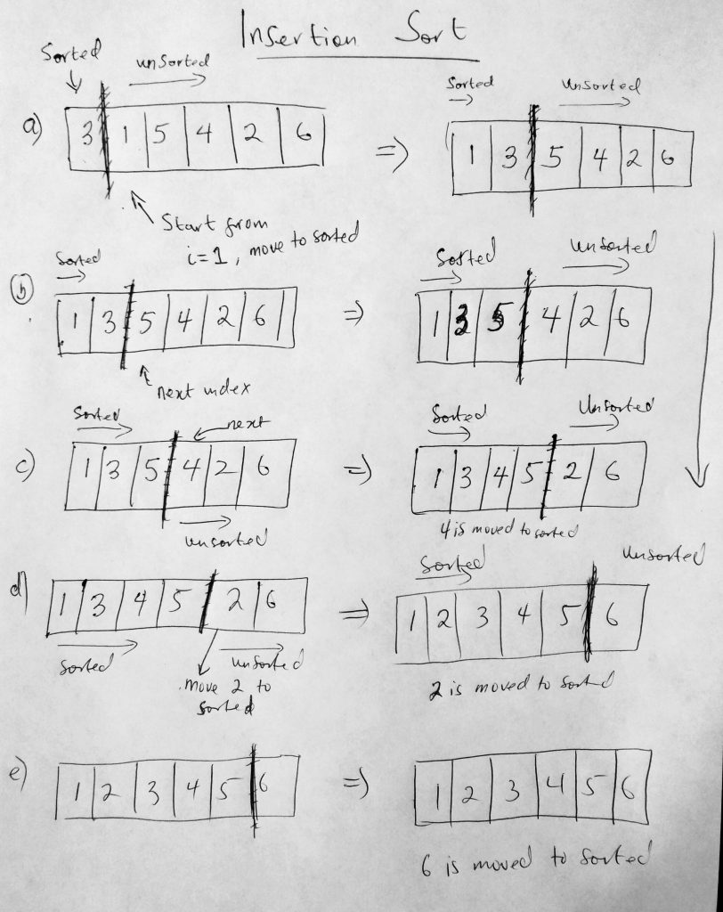
Taking a look at the diagram, we start of by defining the sorted and unsorted areas of the collection. Notice that the sorted area has only one element (hence a size of 1). The first item is considered the sorted section, the rest are all unsorted. The idea is that we start from the second item and move it over to the sorted section. In this case 1 is less so we put it before 3. We move to the next item in the area and bring it over to the sorted section (into its right place). We keep doing this till the collection is sorted. Now that you have a better idea of how insertion sort works, lets take a look at the code.
See the Pen Insertion Sort by kofi (@scriptonian) on CodePen.
Lets walk through what is going on in the code. Notice that the outer loop thats from i = 1. This is so that we start from the second item in the collection (which is the first item in the unsorted section). We store that item in a temp variable as well as its index. This is so that when we insert it on the other side we know value value it is. We also want to know its index so we can shift other items into its slot ( a placeholder ). The hardest part of this algorithm is what happens in the inner loop. As long as the placeholder is greater than zero, and the last item in the sorted section is greater than the temp variable we are holding, we keep shifting the items over into the placeholder and into the slot before that etc. When the conditions are no longer met it means that we have found where to insert our temp variable, we exit the while loop and insert in that placeholder. Please take a look at the code for further clarification but i hope that helps. I have provide an alternative method for doing insertion sort using 2 for-loops instead of one for, and one while loop (just to see why one you like better). You might find that simpler to understand. In any case, do poke around the source code on github.
Now lets take a look at how this algorithm performs. In the worst case scenario it performs at O(n^2) for data sets that are large, even though all the sorting happens in one pass. The performance hit comes from selecting the right insertion location and all the data shifting around. Remember when you insert data, you have to shift everything after it to the next slot. The average is also O(n^2). Best case is when the data set is low or already sorted or nearly sorted data. The big O notation for best case is O(N). Space complexity is O(N), which is not bad. This is because we don’t need to allocate extra space when doing insertion sort. If minimizing memory space is important, algorithms like these are useful. It is also worth mentioning that faster algorithms (which follow a divide and conquer approach to sorting collections of data) use insertion sort internally for smaller collections. Finally insertion sort is a stable sort (order of elements are maintained).
We have looked at 3 basic sorting algorithms. Lets turn things up a notch and look at a few advanced sorting algorithms. Algorithms that give us much better performance than the basic ones.
Advanced Sorting Algorithms
Lets kick things up a notch by moving away from algorithms that have a time complexity of O(n^2), as these are not the best. The next 4 sorting algorithms are more real world, and are more likely to get used. We will talk about are shell, merge, quick and heap sorting algorithms. We will start from order of increasing performance and code complexity/difficulty. Lets start with the shell sort.
Shell Sort
The last basic sorting algorithm we looked at was the insertion sort. The Shell sort algorithm (named after the inventor Donald Shell) uses insertion sort extensively. So insertion sort is at its core. However it adds something very “smart” in order to achieve a far greater performance than insertion sort. The runtime complexity lies somewhere between O(n) and O(n^2). And space complexity is O(1) as the sort is in place and doesn’t take addition memory.
So how does this it work? Shell sort breaks apart the original list , into smaller sublists. The sublists are made up of elements from the original list separated by an increment value. Maybe an example will help. Take this array list
[1, 5, 3, 4, 2, 6]
Given a starting value of 0 and an increment of 2, the algorithm will first pick the 1, 3, and 2 elements (since they separated by an increment of 2) and sort that first. This increment is also know as a gap. Let me mark those values with an asterisks *
[1*, 5, 3*, 4, 2*, 6]
This is the first sublist that the algorithm will do. When this sublist is made (in memory) it will be sorted in ascending order.
[1, 5, 2, 4, 3, 6] – after sort
When that happens, notice that the 2 and 3 have changed positions. Then it moves to the next sublist which start at index 1 (remember the first sublist started from 0 – we are moving through the entire list based on gaps/increments)
[1, 5*, 2, 4*, 3, 6*]
I have marked the second sublist with * this time. Once the algorithm has this list, it will sort that as well. Once sorted we have this
[1, 4, 2, 5, 3, 6] – after sort
There are no more sublists that can be created. The idea is that at this point the array is nearly sorted. Remember the nearly sorted arrays could potential have a runtime complexity of O(n). And that is the whole point of this algorithm. To get to a point where its almost nearly sorted so the final sort happens swiftly. By performing the earlier sublist sorts, we have reduced the total number of shifting thats needed to be done on the list. Lets take a look at a diagram.
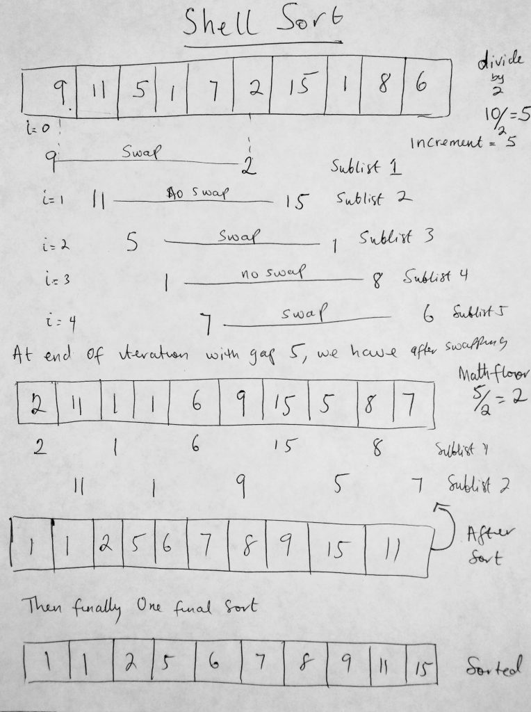
Notice in this diagram that we sort first using an increment of 5 (top right edge of image). This is different from the first insertion algorithm with did which used the default increment of 1. How did we get 5? Well we divide the total number of items of the collection in half (there really isnt a set rule here, as all we are trying to do is come up with an interval schema). After we are done sort with 5, we divide it by 2 again, and take the Math.floor value, which is 2. Then we sort again using that gap. After that we divide the increment by 2 again (2/2 which is 1). Then we sort the entire list with a gap of one (which we are already accustomed to doing). Ok, lets look at the code for this.
See the Pen Shell Sort by kofi (@scriptonian) on CodePen.
Since we have already looked at insertion sort, the code above should be be pretty clear. I have provided two insertion sort methods like i did previously. This insertion sort however takes into account the increment or gap that should be accounted for when doing shell sort. When we call shell sort, like we call all sort functions, we pass it a data list. With this list we write an algorithm that determines what increment value we will use to generate our sublists. What use an approach of always dividing the data list length. No need to speak about this again since i explained it before we saw the code. What we can add upon that is while that increment is greater than or equal to one, we call our new version of the insertion sort passing it the data list, the start index and the increment value. With these parameters the new insertion function can create sublists and do its sorting magic. We keep sorting till we get to an increment of 1 (which is nearly sorted). After that sort we are done. I provide two methods for you just for convenience. You can either call the insertionSortGap or the insertSortGapAlternative. Choose whichever style is comfortable for you. Or share with me your approach (i am always happy to learn other techniques, they can only make me a better developer). Ok lets move onto the next sorting algorithm.
Merge Sort
Merge sort is the first algorithm we will look at that uses recursion. We first looked at recursion when we studied binary search trees. The process in which a function calls itself directly or indirectly is called recursion, and the corresponding function is called as recursive function. Merge sort is a divide and conquer algorithm. By recursively breaking down a problem into two or sub problems of the same or related type, they become simple enough to be solved. The performance of merge sort is great, with a time complexity of O(n log n). This is the best we have seen for worst case scenario. But as you will see later on even the best case scenario is O(n log n). You might think, we have seen better best case scenarios in other sorting algorithms. One of the “so called” slower algorithms had a best case scenario of O(n). Merge sort blows them away with worst and average case scenarios O(n log n) versus O(n^2) – which makes it a winner overall. You might be interested to know that Firefox uses an implementation of merge sort. Chrome uses a different sorting algorithm (quick sort). It is always a good idea to have a working knowledge of how these sorting algorithms work. You might want to use one over the other (it all depends on what your application needs are). Its cool to know that if you were every in the console and wrote a function that uses the internal sort function, that you know which implementation it is.
So what happens in merge sort? We use recursion to split the data list in half. The splitting continues until there are only groups of 1. So an array with 8 items gets split to 4, then 2, then 1. At that point, it is reconstructed. The data list is put back in sorted order by merging the groups (the array doubles in size during this merge from 1, 2, 4 and finally 8). Lets take a look at a diagram.
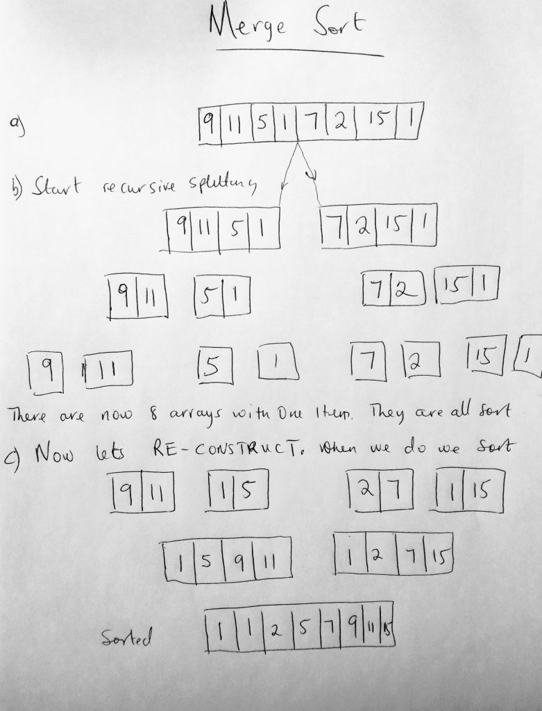
I think its much easier to understand with the diagram right? We break the array apart till there are only single items in the array. So at the end of the splitting, we have 8 arrays with a single item in them (which means they are sorted – only a single item). From here we start constructing them back to a whole. However when we do, we sort them in the process. At the end of the construction, we get an array with all the data sorted. Lets code this out. And talk more about performance for this algorithm.
See the Pen Merge Sort by kofi (@scriptonian) on CodePen.
The merge sort algorithm is split of several helper methods. First we have the main call to mergeSort which then calls the mergeSplit method. The split method is responsible for splitting up the data list into sub modules recursively. As the splitting occurs the merge function is called at the end of the call stack and starts the reconstruction phase. I think the recursion part is the hardest part to understand. Recursion is quite deep, and on first glance you might react with the “what the hell” remark. Even more experience engineers need to really look at the code to truly see what is going on. Perhaps i should do a post on recursion? Check this tutorial out in codecademy (i highly recommend it). The merge function is probably the simplest to understand. The function takes in a 2 arrays as parameters. As long as there is data in either of the lists, it checks the first item in both them, whichever is smaller gets added to a results list (a list that sort in increasing order). At the end of the while loop, one array will be empty and chances are the other array will have either 1 or many items within it. All we do is concatenate those items to our results array and return it. Let move to the next sorting algorithm.
Quick Sort
Quick sort is probably by far the most widely used general-purpose sorting algorithm. Googles chromes javascript runtime uses quick sort as the preferred sorting algorithm. The C and C++ standard libraries also use quick sort. It is a divide and conquer algorithm and therefore involves partitioning of data into smaller subsets. Where merge sort takes the approach of recursively splitting data in half, in quick sort, we pick a pivot value, and put values that occur before that pivot to the left of it, and all values above to the right (you can think of the pivot as helping to split the list). This is the partitioning aspect of quick sort. The lower values are partitioned to the left and higher to the right. A pivot value is sometimes picked based on a certain rule, but there really isn’t a right way or science to pick a pivot value. However based on how your collection is structure there might be better pivot values one can choose. Usually however we could pick the first or last element of the sublist. Lets get back to the discussion of pivot partitioning in quick sort. After the first partitioning is done, we perform the operations again on the left and right partition. We keep doing this until data is sorted. A picture is worth a thousand words, so lets take a look at a diagram that will give the description here more meaning.
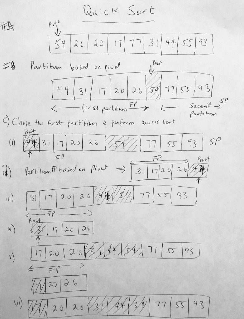
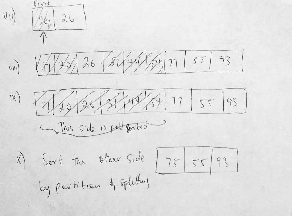
Above is a visualization of quick sort. Given a list, we first find a pivot. In our diagram, we chose 54 as the first pivot. once we have found the pivot we go through the entire list and move elements that are smaller to the left and elements larger to the right. In B of our diagram, we can see that we have moved all values that are less than 54 to the left of it, and all values bigger to the right. Please take note, how these number are arranged does not matter as long as the lesser values are on the left and the greater value on the right. For example the first partition has number 44, 31, 17, 20 and 26. Those could have been rearranged differently. like 17, 26, 20, 44 and 31. It doesn’t matter. What matters is that they are to the left of 54. Now that we have two partitions we break them even further. Lets start with the first partition. Now that we have two partitions we can further partition both sides. In figure C, we take the first partition, choose a new pivot point. We choose the first item in the first partition which is 44, and after sorting it we get what you see in the figure C iii. We pick the next sublist and pick a pivot point (iv). We sort that to get (v). Notice that when we get to v and we choose 17 as a pivot we only get a partition that we can sort on the right instead of the left. This is how we got the result in (vi). In (vii) we make a sublist out of that are partition. Hopefully you see the pattern now. We keep doing this until the first side is fully sorted. Then in (x) we repeat this again for the other side. Lets code this out and complete it by looking at performance features.
See the Pen Quick Sort by kofi (@scriptonian) on CodePen.
I must say the code here is quite hard to code. However if you have understood the inner workings of quick sort, then it shouldn’t be too bad to understand as the code does exactly what we have already talked about. I also suggest you watch this video on quick sort (its one of my favorites on quick sort). Lets summarize the code. Our implementation is split over 3 helper methods. The main or entry point is the quickSort function. We pass in a data list as a parameter. From there we take the high and low values of that data list and pass that to our recursive function. We need the high and low values to get our pivot points. Remember this can be any element in the array. From the examples we looked at earlier, we always used the first element of the sublist. The first thing we do is get the pivot point by calling the partition method with our data list and high/low values. Notice here that we are using the low value. We could have used a random value (which some say is best) or even chosen the middle value. I will let you decide on how that pivot value is determined. We then perform our partitioning as long as the low and high do not cross each other. In the partitioning we find elements that are less than the pivot and we put that to the left side, and the ones that are greater to the right side. Thats what the partitioning logic is doing. The inner while loops determine new high/low indices and based on that does a swap. At the end of the method we return the low index, which becomes our pivot for the next iteration of sublists. Another way to process the partitioning logic is this, once a pivot value is picked all the values in the array that are smaller are placed on the left and all the larger values are placed on the right. When we do this we have 2 partitions. Each partition will be partitioned further. This is repeated over and over again till the data is sorted. There is really no easy way of explaining quick sort. Whew! That was a tough one. So far i have found quick sort and finding the shortest path in graph algorithms probably the hardest to code and understand (took a lot of time). Another one on the list is heap sort which we covered next. That too is hard to code!
Lets talk about performance. The running time complexity is O(n log n) for average case scenarios. This is pretty good for a sorting algorithm. You will be surprised that it runs at O(n^2) for worst case scenarios. You will find this for large data sets that are nearly sorted. For best case scenarios we still have O(n log n). Space complexity for quick sort is O(n) as array and stack space must be considered. Quick is preferred to merge sort for a few reasons that has nothing to do with runtime complexity. It seems the locality for references reading from cache is much better in quick sort. If you have a constraint on time, you typically use quick sort (which is generally the case) – space is not really an issue these days, its time. Finally it is not a stable sort. Lets move to the final sorting algorithm.
Heap Sort
To under heap sort, one must first understand the heap data structure. I just wrote a post on it just so that this section isnt too long. So read it here first before continuing with this post. This sorting algorithm uses the help of a heap data structure to sort elements in a collection in ascending or decreasing order. It does so by converting the collection/array into a heap (which is all done in place – no extra memory is needed). From here we can access the highest element in the heap, remove it and put it at its right location (the end of the array). So the second part involves converting a max heap into a sorted array. To recap, the first phase involves heapifying and the second is sorting. Please be sure to read the other post (if this is sound gibberish), as i will be skipping some of the theory already covered. The code for heapsort is a bit involved as it borrows code from our heap implementation.
Ok, lets talk about the code here. Some helper methods we use here is get left, right and parent index (like we have for our heap class). We make some changes to trickledown method. After we get the right and left child indice, we do some checking to make sure that the left and right child satisfiy the max heap property (since we are using a max heap implementation). If this property is not satisfied we perform a swap. Each time we perform a swap, we trickledown and check to see if the remaining elements are also satisfied. The heapify method takes the last index in the heap, gets its parent and trickledown the node. The second phase takes the heap and transforms it into a sorted array. This is all done in place. Take a look at the code
See the Pen Heap Sort by kofi (@scriptonian) on CodePen.
Now that we see how to implement heap sort, lets take a look at the runtime complexity for this sorting algorithm. Some of the operations that happen N times are, insertion into the heap, removal of maximum elements followed by heapify. Since these operation already operate at Log N, we get an average case scenario is O(N log n). Which is the number of times multiplied by log N. There is no addition space needed, so space complexity is O(1). Other things to note about this algorithm is that its not adaptive. If the heap is almost sorted it wont go any faster. Another thing to note is, its not a stable sort.
OK! Thats all folks. I have really enjoyed first of all learning these algorithms and sharing it with you. I know i rushed over the heap sort part (but its only because there is an entire post i write just before i could finish this post). If there are any questions, please ask and i will do my best to get back to you. Feel free to reach out on twitter as well ( @scriptonian ) if you have any questions. Let’s write our final post in this series by learning how to implement so well know advanced algorithms in javascript.